Emacs Calc Tricks
I've been learning and using the advanced RPN calculator included in
Emacs, known as calc. The primary reason is that it is aware of
units. As they say, a number without a unit is meaningless, and it
now baffles me that so few programming langauges care to track them at
all. It's also built-in to my favorite text editor, which makes
copying data in and out of calc very easy. And along those lines,
it's a useful tool with org-mode tables, turning them into mini
spreadsheets.
Like Emacs itself, calc is a deep and intimidating tool. But after
getting comfortable with a few basics it's easy to learn more advanced
features from the built-in info documentation.
Stand-alone calc launcher
I like calc so much that I recently replaced the Galculator launcher
in my desktop environment with this script:
#!/bin/sh
emacs -g 40x20-0-0 -eval '(progn (calc) (message "") (delete-other-windows))' &
This starts a small Emacs window in the bottom right corner of my
screen and clears the default welcome message. I also have the
following snippet in my .emacs.d/calc.el file so that the paper
trail isn't displayed:
(setq calc-display-trail nil)
Mibibytes
I recently did some work defining partition table sizes, and it was
useful to define these units in my calc.el:
(setq math-additional-units '(
  (GiB "1024 * MiB" "Giga Byte")
  (MiB "1024 * KiB" "Mega Byte")
  (KiB "1024 * B" "Kilo Byte")
  (B nil "Byte")
  (Gib "1024 * Mib" "Giga Bit")
  (Mib "1024 * Kib" "Mega Bit")
  (Kib "1024 * b" "Kilo Bit")
  (b "B / 8" "Bit")))
(setq math-units-table nil) ; Clear the units table cache
(Lifted from: https://www.reddit.com/r/emacs/comments/31xezm/common_byte_units_in_calc/cq6ef06/)
Curve fitting in calc
What really convinced me to stick with calc mode was a recent struggle with LibreOffice Calc. I wanted to do a polynomial curve fit of some data (to use as input into a circuit simulation), but after I setup a chart and plotted the fit, I was unable to copy the formula as text. If I attempted to paste it in another program it would paste as an image. This was less than helpful.
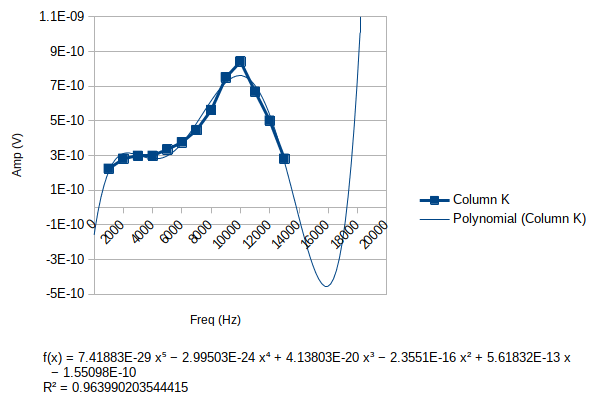
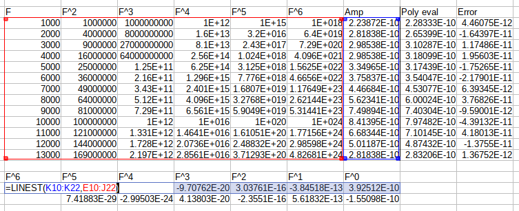
The workaround for LibreOffice Calc was to learn and use the LINEST
function, which is an array function. That was a new trick for me,
but it certainly wasn't intuitive to setup, and the output wasn't in a
particularly useful format. There was one coefficient per cell, but
no labeling for which term the coefficient applied to, and in fact the
coefficients were in reverse order from the way I supplied the terms
to LINEST. I was not happy with this solution.
A bit of research showed that calc could find and plot curve fits as well: https://www.gnu.org/software/emacs/manual/html_mono/calc.html#Curve-Fitting
The input points can be entered as a Nx2 matrix like below, and then
transposed into the format calc expects with v t ("vector,
transpose").
[
[ 1000,lufquant(-193.5dB,1)],
[ 2000,lufquant(-191.0dB,1)],
[ 2500,lufquant(-190.0dB,1)],
[ 3000,lufquant(-190.5dB,1)],
[ 4000,lufquant(-190.5dB,1)],
[ 5000,lufquant(-189.5dB,1)],
[ 6000,lufquant(-188.5dB,1)],
[ 7000,lufquant(-187.5dB,1)],
[ 8000,lufquant(-183.0dB,1)],
[ 9000,lufquant(-182.5dB,1)],
[10000,lufquant(-181.5dB,1)],
[11000,lufquant(-182.0dB,1)],
[12000,lufquant(-183.0dB,1)],
[13000,lufquant(-190.0dB,1)],

[15000,lufquant(-194.0dB,1)],

[18000,lufquant(-200.0dB,1)],

[20000,lufquant(-250.0dB,1)]
]
The lufquant is a calc function that will convert a decibel value
(\(20\log_{10}(x)\)) into the corresponding field quantity, with default
reference and units set by the calc-lu-field-reference variable in
Emacs. But here I'm passing in a unitless `1` to do the ratio
calculation without units.
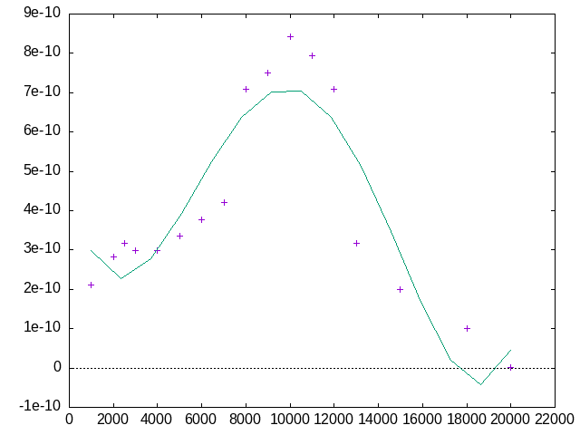
The a F command will take a 2D matrix of data (2xN), then ask what
type of fit you would like to perform. I entered "P" to request a
graphical plot using gnuplot, then "5" for a 5th order-polynomial fit,
and finally entered "F" to be used as the variable of the polynomial,
and calc output a polynomial in a convenient text format. Minimal
edits allowed that to be understood by my circuit simulation program,
and I now had a voltage source whose amplitude was a function of the
simulation frequency.
3.64573332806e-31 F^5 + 1.20125808335e-25 F^4 - 5.36854825319e-21 F^3
  + 6.69611214816e-17 F^2 - 2.32309953748e-13 F + 4.68451430373e-10
And it even generates a plot of the input data and the fit at the same time. Very handy.
Update
This gets even better with WebPlotDigitizer, which I just read about in XKCD #2341. WebPlotDigitizer lets you upload a graph, click two points on each axis (X and Y), specify if they are logarithmic or not, and then automatically trace a plot based on it's color.
Using the following data from WebPlotDigitizer, I get this graph for an 8th degree polynomial fit:
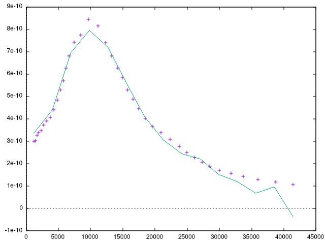
I think it did a better job than I did…
Here's the data, after trimming some of the lower frequency points
and getting it ready for calc (v t a F P 8 F <enter>):
[
[1206.658901024318, lufquant(-190.46560392572664dB, 1)],
[1417.471187673314, lufquant(-190.3630806820991dB, 1)],
[1665.1139490856867, lufquant(-189.72683349370467dB, 1)],
[1956.0217431937924, lufquant(-189.4222791523405dB, 1)],
[2297.7532930690713, lufquant(-189.16597104327167dB, 1)],
[2699.1878869347897, lufquant(-188.56289313958027dB, 1)],
[3170.756090722092, lufquant(-188.14375399651473dB, 1)],
[3724.7107678258976, lufquant(-187.809045759966dB, 1)],
[4311.86372182869, lufquant(-187.11148565136295dB, 1)],
[4847.5578865851, lufquant(-186.30436639025598dB, 1)],
[5331.44717626, lufquant(-185.54147284208634dB, 1)],
[5778.431510723953, lufquant(-184.8979887188476dB, 1)],
[6217.219580237294, lufquant(-184.06875660127196dB, 1)],
[6640.546443020515, lufquant(-183.3440077305108dB, 1)],
[7411.108515269597, lufquant(-182.57432955592466dB, 1)],
[8454.70379670961, lufquant(-182.21980590254034dB, 1)],
[9645.252952755549, lufquant(-181.46768160265094dB, 1)],
[11165.703563910034, lufquant(-181.78228724240995dB, 1)],
[12370.48776254165, lufquant(-182.60930807433877dB, 1)],
[13309.846900776742, lufquant(-183.34566619474597dB, 1)],
[14216.106629891186, lufquant(-184.0571473516259dB, 1)],
[14963.42590478183, lufquant(-184.67907143980764dB, 1)],
[15750.030626325619, lufquant(-185.50830355738333dB, 1)],
[16577.985971175312, lufquant(-186.2380278208499dB, 1)],
[17449.4656792043, lufquant(-187.01750601137104dB, 1)],
[18501.67814519684, lufquant(-187.92966134070429dB, 1)],
[19617.33960693196, lufquant(-188.7340164947527dB, 1)],
[20953.072843434187, lufquant(-189.4156452953999dB, 1)],
[22379.755378610287, lufquant(-190.2100496640374dB, 1)],
[23729.26705009381, lufquant(-191.10562035101913dB, 1)],
[24976.67881389389, lufquant(-192.0315962156453dB, 1)],
[26097.952158352404, lufquant(-192.84977190498662dB, 1)],
[27269.562616178202, lufquant(-193.701116879031dB, 1)],
[28493.769961934435, lufquant(-194.49717971190364dB, 1)],
[29991.64445466525, lufquant(-195.32641182947933dB, 1)],
[31800.15726250572, lufquant(-196.11418234117622dB, 1)],
[33717.724396495825, lufquant(-196.84390660464283dB, 1)],
[36013.54462686531, lufquant(-197.7477696128003dB, 1)],
[38748.25104223567, lufquant(-198.52393087485112dB, 1)],
[41386.596904136204, lufquant(-199.42281849030317dB, 1)]
]